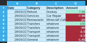
1. Select your whole table including headers

2. With your table selected, go to Data > Pivot Table > Insert or Edit…
3. Select Current selection for Selection then click OK
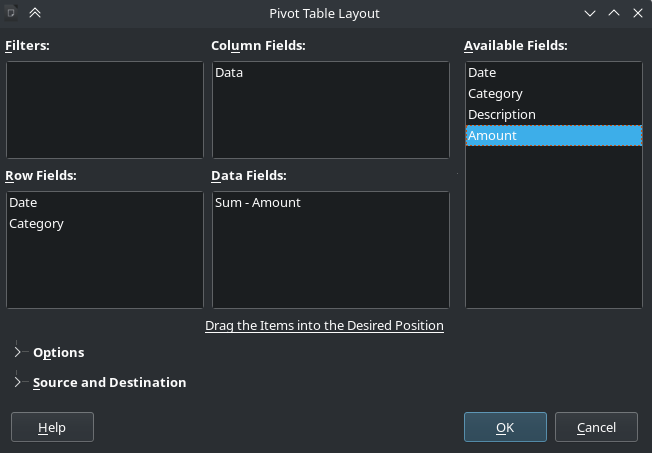
4. On this page, you can drag the available fields to any box you want (Filters, Column, Row and Data). For what I am doing I will drag my headers into these boxes and click OK:

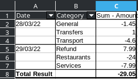
This will create a new sheet by default with this:

Now we will group the dates by month and year, but feel free to group them however you like.

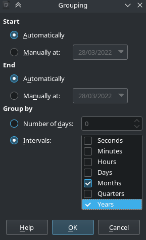
1. Click the first cell under the filtering box (in this case A2) and go to Data > Group and Outline > Group (or press F12).
2. We can keep everything default, except I am going to make sure Months and Years is selected under Intervals in the Group by section and click OK:

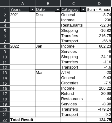
This is what your pivot table should now look like (I added more data):

• If you right click anywhere on your table and go to properties, you can tweak your table.

• Double clicking fields (in this case, like Amount, Category, etc) allows you to modify how their values are presented.

• You can go under Source and Destination to increase the source selection range which will allow you to include more rows, if you add them down the line.

• To update the data displayed in your pivot table you can right click > refresh on it.